Finance is arguably the largest and hardest area of knowledge work. Accurate predictions of the global financial market drive trillions of dollars of value, and take the best experts many years to hone, and even then imperfectly.
A couple of months back, we created a research effort at Samaya to study AI’s predictive capabilities in finance. Making accurate financial predictions requires access to a large set of high quality, real-time financial information — finance’s “open-world” equivalent of a codebase. We built a finance-specific prediction harness and environment to give AI models comprehensive, point-in-time financial information at parity with human experts so that we could push their capabilities to the limit.
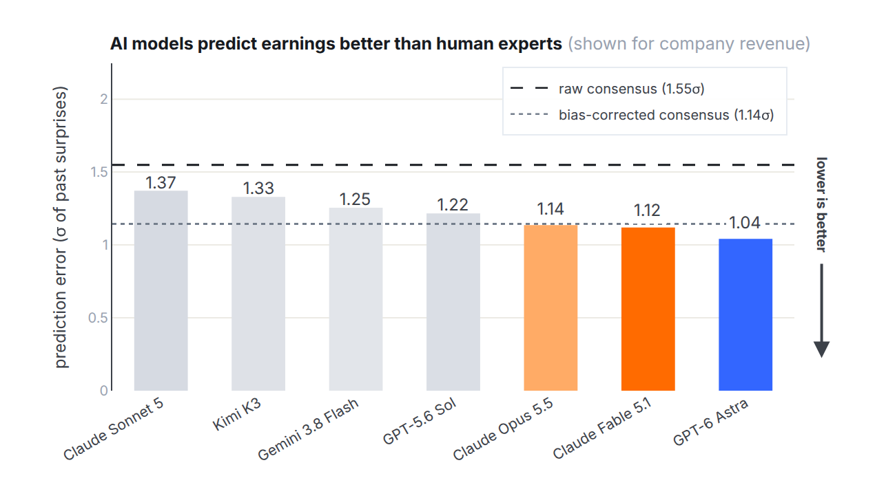
Our results show that we have reached a critical inflection point. For the first time, we see that the latest frontier AI models working with Samaya’s finance harness outperform human experts in financial prediction. Specifically, we find that the latest AI models outperform expert analysts in predicting earnings surprises.
Earnings predictions and surprises
Global stock markets are worth more than $150 trillion and are the most closely watched asset class in the world, for professionals and individual investors alike. More than ten thousand public companies make up the investable universe across global markets, and most of them report earnings results every quarter, sharing metrics such as revenue, gross margin, operating income and adjusted EPS, also referred to as actuals. These metrics are the foundation for investment decisions into these companies and so an enormous amount of analyst time is spent on modelling, predicting and publishing these metrics ahead of earnings. The average of these predictions is called the consensus estimate.
Consensus estimates form a market baseline for the expectation of a company’s performance. When the company reports, the actual is either a “beat” (above consensus) or a “miss” (below consensus) with the gap being the earnings surprise. Because predicting earnings is extremely challenging, and even the best consensus estimates miss, the market can react strongly to earnings surprises. So consensus estimates provide a strong “feasible” expert baseline to evaluate AI’s ability to predict earnings and earnings surprises.
Building the environment and harness
Besides being a very important task for investing, earnings prediction is also a great task for AI. Not only do we have ground-truth actuals and a consensus human baseline, we also have surprise drivers revealed by the company management which can help us understand if the models’ reasoning process was correct. The earnings prediction task advances financial reasoning: it tests the ability to understand company fundamentals, do deep search and retrieval on competitors, supply chain and macro factors, identify key drivers, make the right assumptions and account for them appropriately.
1. Task environment
In the earnings prediction task, we run the models under Samaya’s harness and make predictions one week before earnings. Through our harness, we provide access to all financial sources available until that point in time. We ask the models to predict four headline metrics: revenue, gross margin, operating income and adjusted EPS. These metrics track the flow of money through the income statement and capture essential aspects important for financial analysis (described in Appendix B). We call each such prediction task, predicting all four metrics for one company ahead of one earnings release, an instance.
To compare the AI models, we calculate three performance metrics (precise definitions in Appendix C):
- Prediction error measures how far the predicted numbers are from the actuals.
- Surprise correlation measures if the surprise (i.e. actual − consensus) is correlated with the predicted surprise (prediction − consensus). This is an overall metric that measures the ability of models to predict big beats and misses correctly.
- Hit rate measures if the prediction and actual are on the same side of consensus.
Normalizing for volatility: Because some companies’ financials vary more than others, we normalize by each company’s historical surprise volatility to make the predictions comparable across companies.
Building a harder expert baseline: We found the consensus baseline relatively easy for AI models to outperform. This is because analysts systematically lower their estimates ahead of earnings,1 so actuals beat the consensus more often than not. We wanted to measure the ability of AI models beyond simple corrections like this, so we created a harder bias-corrected consensus baseline by adding each company’s historical median surprise.
2. Samaya’s prediction harness
To evaluate models on this task, we needed to be able to run multiple experiments by rewinding time and restricting access to future information. To build Samaya’s prediction harness, we started with our production harness and modified it for this environment.
- 1Production harness. To begin with, Samaya’s production harness provides context-efficient financial retrieval over unstructured and structured data sources used for real-world investment decision-making.
- 2Point-in-time gate. Then, we introduce a point-in-time gate enforced at the harness layer. This gate is enforced programmatically with an authentication token that prevents any possible hacking or cheating by the model.
- 3Time-aware retrieval and data tools. We modify our retrieval stack to respect the time-based cutoff, and we re-create some of our structured data tools to support this gate as well.
- 4Substituted web access. We remove web access because it is very difficult to apply a point-in-time gate to it. Instead, we add essential news sources behind the gate, which are a reasonable proxy for web access for this task.
- 5Expert guidance. Finally, we modified our harness to increase context efficiency and added expert-guided instructions to improve predictive reasoning.
In our experiments, we tested seven frontier models: GPT-6 Astra, Claude Fable 5.1, Claude Opus 5.5, GPT-5.6 Sol, Claude Sonnet 5, Gemini 3.8 Flash and Kimi K3. We chose companies that reported from July 14th onward (after the knowledge cutoff for all models) with more than $5 billion in market cap and more than 8 brokers providing estimates, leading to 456 companies that cover all sectors.
AI outperforms consensus in predicting earnings surprises
Our main results show that frontier AI models using Samaya’s harness are able to outperform consensus. Even older, smaller models such as Sonnet 5 and Kimi K3 outperform raw consensus, but only the most recent models (Fable 5.1; Opus 5.5; GPT-6 Astra) are able to outperform the harder, bias-corrected consensus baseline — highlighting a key inflection point in AI capabilities. We find GPT-6 Astra to be the highest performing model across the most metrics (prediction error for revenue (Figure 1), overall prediction error, hit rate), but we see some variation in model performance (Fable 5.1 and Opus 5.5 best performing on surprise correlation).
We looked at some of the traces produced by Claude Fable 5.1 and GPT-6 Astra (the top two models) under Samaya’s prediction harness and analyzed the reasoning process they followed. We find that the models are able to calculate the financial impact of world events and news the way we expect from a strong human analyst. In fact, anecdotally, the models’ ability to gather new evidence and willingness to adjust their view away from the consensus drive their wins over consensus.
Disentangling the impact of the data, harness and model
We carried out an ablation study to understand the individual components of our system and their contribution to model performance.
Access to live data is the most important factor in accurate financial predictions
Here we compare three settings: (1) no data, i.e. the model relies purely on parametric memory; (2) stale data, by asking the models to make the same prediction 11 weeks in advance, i.e. within a couple of weeks of the previous earnings call; and (3) the latest data.
- As expected, even the best models struggle without access to any data. In particular, we see that Claude Fable 5.1 (knowledge cutoff June 26) is unable to utilize publicly available information in its parametric memory.
- Giving models access to the data at the beginning of the quarter raises performance by 25pp, underscoring the importance of having access to real data.
- But there is still a 12–16pp gap with the full data setting, roughly equivalent to the difference between Claude Sonnet 5 and Kimi K3 vs the frontier models. This also corroborates the observational evidence in the previous section that models do well by finding timely information and updating their estimates.
Expert guidance strengthens search and reasoning
We also ablate the effect of expert guidance, finding that with expert-guided instructions models research roughly 1.6–2.7× more (in time spent and context used), leading to reductions in model error.
The best models do well even when the consensus is taken away
While using consensus and improving upon it is standard practice for traders and portfolio managers, we also wanted to measure AI performance when it cannot see the consensus at all. We created a new set of tools that eliminate all structured sources of estimates and redact any sentences in the retrieved documents that give away consensus figures.
We found that the weaker models benefit a lot from having access to consensus, whereas the gap narrows with better models. In particular, GPT-6 Astra achieves nearly identical performance, possibly reconstructing the consensus from publicly available information.
What’s next?
Our results show an exciting advance in AI for finance: frontier AI models, given the right harness integrated with financial data, are able to outperform experts at prediction tasks such as earnings surprises.
- Try out the predictions and adapt them to internal data. We have an alpha version of the earnings prediction agent within the Samaya product available for users and clients. We’re also working with clients on adapting these predictions to internal data to generate firm-specific insights. Get in touch to try it out and collaborate!
- Further research on modeling reasoning. How do these models make the predictions? Are they able to identify the actual drivers reliably? Are they less biased compared to human analysts? Can we complement human reasoning with AI reasoning mechanisms? We’re researching these and other related questions.
- RL post-training and continual learning. The earnings prediction environment provides high quality signal for RL training and we’re working on training AI models to learn from their past mistakes on this and other predictive tasks.
Acknowledgements
We thank Richard Diehl Martinez and Rajul Bothra for their contributions to designing the environment, and Yuhao Zhang, Ozan Koyluoglu and Thejas Venkatesh for their feedback on this work.
Appendix A. Additional results
Frontier models outperform on bigger surprises. The revenue error split by how far the actual landed from the consensus, six models, the three frontier models in colour and the rest in grey. In the two outer groups the bars are sorted by height; the line in each group is the raw consensus.
Understanding the stochasticity of models. We ran GPT-6 Astra and Claude Fable 5.1 five times each on a cohort of 100 companies. We found that while there is variation from run to run, averaging across multiple runs does not lead to significant improvements.
Some metrics are harder to get right than others. The models did better relative to the street on revenue and gross margin than on operating income and adjusted EPS. There are two possible explanations: (1) operating income and EPS are downstream of the other two metrics and can have compounding errors; (2) these are adjusted numbers and different companies have different conventions on accounting for one-off items.
Appendix B. Why we chose the 4 headline metrics
The four metrics follow the flow of money through the income statement. The flow begins with revenue, the goods or services sold by the company. Gross margin is the share of each sales dollar left after the direct cost of making the product. Then we take out the cost of running the business, leaving us with operating income. Finally, adjusted EPS is the per-share profit that ultimately accrues to shareholders, after financing and taxes.
| Metric | What it is |
|---|---|
| Revenue | Total value of what the company sold. The starting point: what the business sells. |
| Gross margin | Share of each sales dollar left after the direct cost of making the product. Revenue minus the direct cost of making the product, as a share of revenue. |
| Operating income | Profit from the core business after the cost of running it. Gross profit minus the cost of running the business. |
| Adjusted EPS | Per-share profit after financing and taxes, one-time items excluded. The number the market reacts to most. Operating income minus interest and taxes, divided by shares outstanding. |
Appendix C. How we score the models
Each is one metric of one instance (one company and one earnings release), with the model’s prediction and the actual reported value .
Consensus. On the prediction day, every broker covering the company has a published estimate for the metric. We take the median broker estimate at the close of that day as the consensus, to prevent skew due to outliers:
Past surprises. For each of the company’s previous eight quarters , the surprise is how far the actual landed from the consensus a week before that quarter’s earnings release, as a percentage of the consensus for revenue and operating income and as a plain difference for gross margin (in points) and adjusted EPS (in dollars):
Bias-corrected consensus. The company’s typical surprise is the median of its past surprises, . We add it to this quarter’s consensus, but only when it is positive, so the correction can lift the consensus and never lowers it: the first form for revenue and operating income, the second for gross margin and adjusted EPS.
Surprise volatility. Some companies surprise by much more than others. Their surprise volatility is the standard deviation of the same eight past surprises, floored at a quarter of the median across companies for that metric, so that a company with an unusually steady history cannot turn an ordinary miss into a huge error.
Prediction error is the distance between the prediction and the actual, in units of the surprise volatility, averaged over all metrics of all instances, with a single metric capped at 10 so it cannot dominate the average: where the scale puts the error in the same units as : the reported revenue for revenue and operating income (a percentage error), and 1 for gross margin and adjusted EPS.
Hit rate is the share of predicted metrics where the prediction and the actual land on the same side of the consensus, leaving out metrics where either equals the consensus exactly.
Surprise correlation first turns the predicted and the actual surprise of each metric into units of the company’s surprise volatility, so that all companies and metrics sit on one scale (both clipped at ±10), where for revenue and operating income and 1 otherwise. It is then the rank correlation between the two across all metrics of all instances, high when bigger predicted surprises go with bigger actual surprises, in direction and size: This is a standardised unexpected earnings measure in the spirit of Livnat and Mendenhall (2006),2 scaled by the company’s own surprise volatility rather than by analyst dispersion.
Significance. Significance marks (†) use a one-sided paired company-cluster bootstrap (companies resampled with replacement, 2,000 draws).
1 B. Baik and G. Jiang (2006), “The use of management forecasts to dampen analysts’ expectations”, Journal of Accounting and Public Policy 25(5), 531–553. ↩
2 J. Livnat and R. R. Mendenhall (2006), “Comparing the post–earnings announcement drift for surprises calculated from analyst and time series forecasts”, Journal of Accounting Research 44(1), 177–205. Our version is scaled by the company’s own past-surprise volatility rather than by analyst dispersion. ↩